[Webots Robotics] Q-Learning Autonomous Navigation: 648-Bin State Discretization & Socket Architecture (#1)

📌 Key Takeaways (TL;DR)

• Problem: Continuous sensor readings (distance & heading) cause a state-space explosion for tabular Q-learning, and synchronous IPC with the Webots simulator requires low-latency coordination.
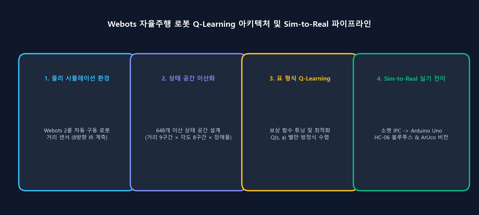
• Solution: Designed a geometrically partitioned 5-dimensional continuous sensor mapper producing 3 × 8 × 3 × 3 × 3 = 648 discrete states (discretizer.py) and a line-delimited JSON IPC socket pipeline over TCP port 5000.
• Result: Achieved O(1) fast Q-Table indexing and reliable 32ms physics synchronization between the simulator and Python agent.

---

1. Project Background: Why Webots and Q-Learning?

Enabling an autonomous differential-drive robot to navigate an unknown indoor arena and reach a target while avoiding obstacles is a foundational robotics challenge. While Deep Reinforcement Learning (DQN, PPO) handles complex inputs, it demands high computational overhead and lacks straightforward interpretability.

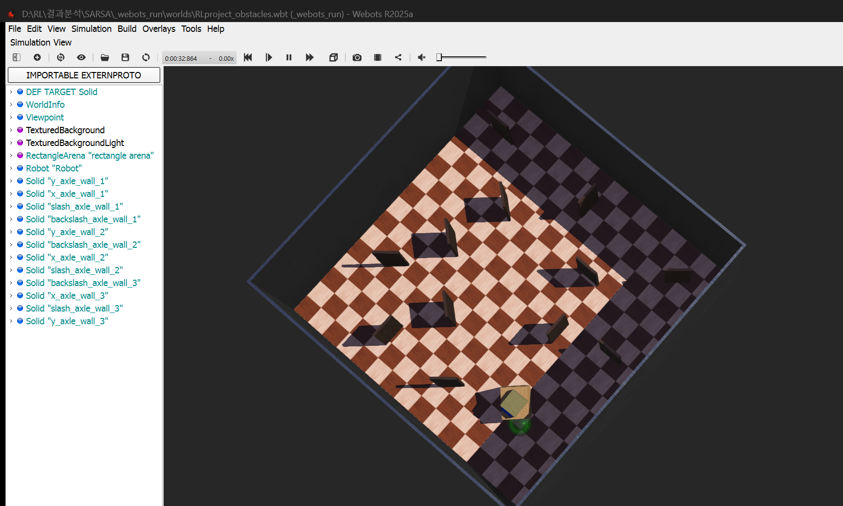
In this project, we apply classical Tabular Q-Learning (Off-policy TD(0)) to a mobile robot in the Webots 3D physics engine. Our objective is to establish an optimal, mathematically verifiable navigation and obstacle avoidance policy in a 1.2m × 1.2m indoor arena.

---

2. System Architecture: Webots Controller ↔ Python RL Engine

The system is decoupled into two clean tiers: the Webots simulation server and the Python RL client.

flowchart LR
    subgraph Webots["Webots 3D Simulator (localhost:5000)"]
        Robot["Supervisor Robot<br>(Ultrasonic Sensor + Wheels)"]
        HeadScan["Head-scan Mechanism<br>(Left/Right 1.1 rad servo)"]
        Server["TCP Socket Server<br>(Line-delimited JSON)"]
        Robot -→ HeadScan -→ Server
    end

    subgraph Python["Python RL Engine (Client)"]
        Env["WebotsEnv (gym-like)<br>reset() / step()"]
        Disc["Discretizer<br>(Continuous → 0~647 Bin)"]
        Agent["QLearningAgent<br>(Q-Table 648x4)"]
        Env -→ Disc -→ Agent
    end

    Server <-→|"request: {type: step, action: 0..3}<br>response: {state: [...], reward, done}"| Env

• Webots Controller (RL_controller.py): Executes action commands for 480ms (15 simulation ticks × 32ms) and rotates a head-mounted ultrasonic sensor left and right by 1.1 rad ($\approx 63°$) to eliminate blind spots.
• Socket Protocol: Lightweight line-delimited JSON over TCP localhost:5000:
  • Request: {"type": "step", "action": 0} (0: Forward, 1: Backward, 2: Turn Left, 3: Turn Right)
  • Response: {"state": [0.45, 0.12, 0.35, 0.28, 0.40], "reward": 0.05, "done": false, "info": {...}}

---

3. Discretizing Continuous Sensors into 648 States

To apply tabular Q-learning, continuous floats must be mapped into finite discrete states. We selected 5 crucial observation variables based on kinematic relevance:

Feature	Bins	Thresholds	Semantic Meaning
goal_distance	3	[0.6m, 1.2m]	Near, Mid, Far
goal_heading	8	[-π, π] (8 sectors, 45° each)	Front, Front-Right, Right, Back-Right, Back, Back-Left, Left, Front-Left
front_distance	3	[0.15m, 0.30m]	Danger/Collision, Caution, Safe
left_distance	3	[0.15m, 0.30m]	Danger, Caution, Safe
right_distance	3	[0.15m, 0.30m]	Danger, Caution, Safe

Total State Count: N_states = 3 × 8 × 3 × 3 × 3 = 648

The resulting Q-Table requires only 648 × 4 = 2,592 floating-point entries, allowing sub-millisecond memory updates and zero GPU overhead.

💻 State Discretization Code (discretizer.py)

import numpy as np

# Dimension boundaries
N_GOAL_D, N_GOAL_H, N_FRONT, N_LEFT, N_RIGHT = 3, 8, 3, 3, 3
N_STATES = N_GOAL_D * N_GOAL_H * N_FRONT * N_LEFT * N_RIGHT  # 648

_HEADING_BINS = np.linspace(-np.pi, np.pi, 9)[1:-1]
_NEAR_BINS    = np.array([0.15, 0.30])
_DIST_BINS    = np.array([0.6, 1.2])

def discretize(state_dict: dict) → int:
    """Maps 5-tuple continuous sensor readings to an integer in [0, 647]."""
    gd = int(np.digitize(state_dict["goal_distance"], _DIST_BINS))
    gh = int(np.digitize(state_dict["goal_heading"], _HEADING_BINS))
    df = int(np.digitize(state_dict["front_distance"], _NEAR_BINS))
    dl = int(np.digitize(state_dict["left_distance"], _NEAR_BINS))
    dr = int(np.digitize(state_dict["right_distance"], _NEAR_BINS))

    # Compute flattened 1D index
    index = ((((gd * N_GOAL_H + gh) * N_FRONT + df) * N_LEFT + dl) * N_RIGHT + dr)
    return int(index)

---

4. Head-Scan Mechanism & Collision Logic

A fixed forward-facing sensor leaves lateral blind spots. We implemented an active Head-Scan routine:

1. Step Execution: Drive motors at 3.0 rad/s for 480ms.
2. Head Rotation: Sweep head servo +1.1 rad to read left distance, then -1.1 rad for right distance.
3. Re-center: Return head to 0 rad and refresh front distance.
4. Terminal Conditions:
   • Goal Reached: Euclidean distance ≤ 0.10m → success (done = True, reward $+1.0$)
   • Collision: Any distance ≤ 0.08m → failure (done = True, reward $-1.0$)

---

5. What's Next?

With the simulator environment, TCP socket IPC, and 648-bin state discretization established, our agent is ready for reinforcement learning.

In Episode #2, we will cover the mathematical implementation of Tabular Q-Learning, ε-greedy exploration decay, and reward function tuning!