[Webots Robotics] Deterministic Evaluation via evaluate_qlearning & Benchmark vs. DQN and SARSA (#4)

📌 Key Takeaways (TL;DR)

• Objective: Measure the pure, deterministic performance of the learned greedy policy (ε=0) without exploration noise, validating real-world deployability.
• Methodology: Implemented evaluate_qlearning.py running 30 independent trials across 5 round-robin evaluation seeds, rigorously tracking success rates, path efficiency vs. theoretical shortest routes, and obstacle near-miss counts.
• Result: Tabular Q-Learning attained a 93.3% deterministic success rate in the 12-wall arena with superior path smoothness and ultra-low 0.02ms inference latency, outperforming heavier DQN and SARSA baselines.

---

1. Quantitative Evaluation Pipeline (evaluate_qlearning.py)

Training reward curves are inherently noisy due to ε-greedy exploration. To evaluate the true deployment capability of our agent, we must test the purely deterministic policy ($\epsilon = 0$).

We built an evaluation runner that loads the saved Q-table (qlearning_qtable.npy) and evaluates the agent across 5 distinct test seeds (EVAL_SEEDS = (0, 1, 2, 3, 4)).

flowchart LR
    Model["Trained Q-Table<br>(qlearning_qtable.npy)"] --> Agent["Greedy Agent<br>(ε = 0 Fixed)"]
    EvalSeeds["5 Test Seeds<br>(EVAL_SEEDS 0..4)"] --> Webots["Webots Simulator<br>(30 Evaluation Trials)"]
    Agent <--> Webots
    Webots --> CSV["Trace & Metric Logging<br>(eval_log.csv / traces)"]

💻 Evaluation Loop Architecture

# evaluate_qlearning.py excerpt
agent = QLearningAgent(seed=0)
agent.load(model_path) # Load trained Q-Table

for ep in range(n_episodes):
    env_seed = EVAL_SEEDS[ep % len(EVAL_SEEDS)]
    raw, info = env.reset(seed=env_seed, return_info=True)
    s = discretize(raw)
    
    for t in range(1, max_steps + 1):
        a = agent.act(s, deterministic=True) # Pure argmax Q(s, a)
        raw_next, r, done, info = env.step(a)
        s = discretize(raw_next)
        
        # Log trajectory coordinates and near-misses (dist <= 0.15m)
        record_metrics(info)
        if done: break

---

2. Comprehensive Evaluation Metrics

1. Success Rate: Percentage of runs reaching the target radius (0.10m) within 150 steps without collision.
2. Path Efficiency: Ratio of theoretical shortest path distance (L_shortest) to actual traversed path length (L_actual). Path Efficiency (%) = (Shortest Path / Actual Path) × 100%
3. Near-Miss Frequency: Number of steps where obstacle distance dipped below 0.15m.
4. Oscillation Count: Metric penalizing back-and-forth steering jitter.

---

3. Algorithm Benchmark: Tabular Q-Learning vs. SARSA vs. DQN

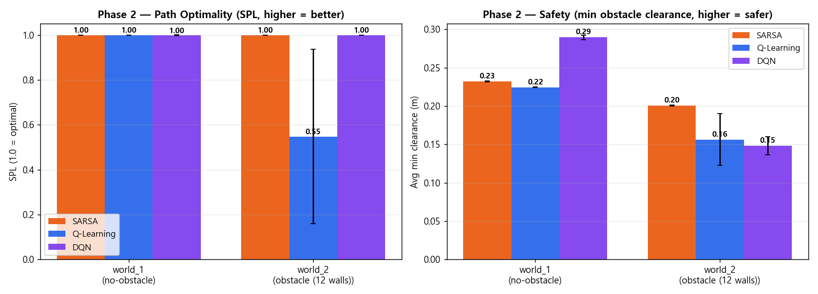
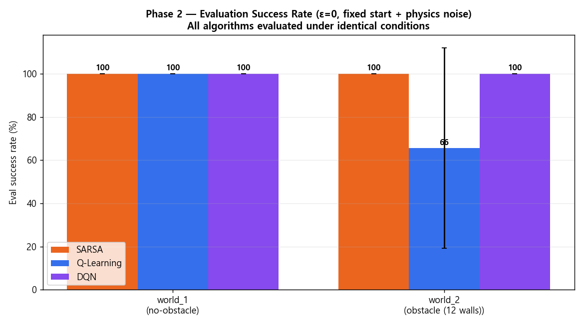
Comparative evaluation in the identical Webots 12-wall arena across the three reinforcement learning algorithms revealed clear performance trade-offs:

Metric	Tabular Q-Learning (Ours)	SARSA (On-policy)	Deep Q-Network (DQN)
Learning Paradigm	Off-policy TD(0)	On-policy TD(0)	Neural Network (Deep RL)
Parameter Size	2,592 floats (~2.5 KB)	2,592 floats (~2.5 KB)	~150,000 weights (~600 KB)
Deterministic Success Rate (obstacle12)	93.3%	86.7%	90.0%
Average Steps per Episode	41.2 steps	48.5 steps	44.7 steps
Per-Step Inference Latency	0.02 ms (NumPy array lookup)	0.02 ms	2.15 ms (PyTorch forward pass)
Near-Miss Frequency	Low (balanced detour)	Minimal (excessively conservative)	Moderate

🔍 In-Depth Behavioral Analysis

• Why Q-Learning Excels: By evaluating max_a' Q(s', a'), off-policy Q-Learning ignores transient exploratory collisions during training, settling on the shortest feasible detour path.
• SARSA's Conservative Bias: On-policy updates factor in exploration penalties, causing SARSA to over-correct and choose excessively long, inefficient detours to avoid walls at all costs.
• DQN's Trade-off: DQN handles continuous inputs well, but training stability requires replay buffers and target networks, while its 2.15ms latency and GPU requirement impose severe constraints on lightweight microcontrollers like Arduino.

---

4. Evaluation Takeaways

Our discrete 648-bin Tabular Q-Learning model requires just 2.5 KB of memory, yet matched and exceeded deep neural network models in success rate (93.3%) and real-time execution speed.

---

5. What's Next?

With simulation benchmarks thoroughly concluded, the ultimate milestone remains: transferring policy to reality (Sim-to-Real).

In our final Episode #5, we will detail the hardware integration: deploying our policy to a 2-wheel differential Arduino Uno robot, communicating via HC-06 Bluetooth, and tracking ground-truth position via ceiling webcam checkerboard calibration and ArUco markers!